![]()
THAT A PORTFOLIO SURVIVES FOREVER
Bernard J. McCabe
Daniel H. Wagner Associates, Malvern PA
We give an approximate formula for the probability that a portfolio with a certain random return and fixed spending survives forever. This is useful as a conservative way of being sure that a portfolio will outlive an individual, no matter how long the lifetime. It could also be used in planning by a charitable trust to ensure that it safely survives.
Key Words: Financial planning, portfolio analysis, Monte Carlo, lognormal distribution.
Introduction
Consider a portfolio which is invested in a way so that the expected return m stays constant over the years, and the spending or disbursements is also constant, corrected for inflation. If the return was not subject to variability or uncertainty then the investor could assure himself that the portfolio would last forever by simply spending less than the return (net of inflation). But realistically the return is uncertain. It may hover around m, and average out to be m over the years, but it varies up and down around m, and the size of the differences is measured by the standard deviation s. There are a number of ways to think about s:
It is also the case that we would like to derive simple formulas for the key event, the probability that the portfolio survives, formulas that can be graphed or used in spreadsheet calculations. Well, wanting to have such formulas and having them are often two different things! But in this case we are fortunate: the formulas can be derived. They are not terribly simple, but they are explicit, and can be programmed on a spreadsheet.
Finally we mention that for detailed planning one may need to resort to a Monte Carlo spending planner such as the one discussed in McCabe (1999). The results here are intended to be insightful, and useful, but they cannot substitute for a detailed examination of an individual’s situation when that involves time varying effects due to variable income and tax status.
The main result
Figure 1 shows our main result, for some typical values of mean return and standard deviation, actually the same values that were analyzed in McCabe (1999). In the figure we show the probability that the portfolio will survive forever as a function of the percentage spending s. That is, s is expressed as a percentage of the initial portfolio value. Note that the survival probability dependence on s is rather gentle, although it does become sharper with the more conservative investments.
There are a couple of interesting things to be learned from an examination of this plot.
![]()
Applicability and Future Research Directions
These results raise some interesting questions for further research.
Suppose we start with a portfolio of size A0. We assume each year i that the portfolio return (as a multiplier) is an independent draw from a lognormal distribution, Li = exp(Xi), where Xi is normal with mean m and standard deviation s, for i = 1, 2, … Suppose each year that an amount s is withdrawn from the portfolio. So the portfolio size in year n + 1 satisfies the stochastic update equation
![]()
It is convenient to assume that A0 = 1 and that s is expressed as a percent of A0. The return m is assumed to be net of inflation. Thus the spending level s can remain constant since it is expressed in constant year 0 currency. Note in the definition of An we do not make 0 an absorbing state – it is unnecessary if we make the convention that An < 0 is equivalent to the portfolio not surviving. This is permissible because once An is negative so are all subsequent values: by definition An+k < 0 if An < 0, for all k, since Ln > 0. Note also that s should represent total spending including whatever will be needed to pay taxes each year.
Under the above assumptions we are interested in calculating the probability a that the portfolio survives forever,
![]()
Expanding the expression for An we have

where
![]()
Note that Mi is also lognormal, but with parameters –m and s. For facts about the lognormal distribution, in particular the formulas for its moments that we will be using, see Johnson and Kotz (1970), Chapter 14.
So,
![]()
and


Since Z = M1(1 + M2 + M2M3 + … ) we see that Z has the same distribution as a random variable of the form
![]()
where M1 and Z* are independent of each other, and Z* has the same distribution as Z.
We can use that equality-in-distribution relationship to set up equations for the first two moments of Z. Those will be used in turn to approximate
![]()
Let m denote the mean of Z and t its standard deviation. Then,
![]()
![]()
and we can solve for m to obtain
![]()
Also, b = E (Z2) must satisfy

and hence
![]()
Monte Carlo experiments simulating the random variable Z show
that its distribution is close to being lognormal. Note that Z is
defined by an infinite sum. We first determined that the distribution of
Z
does not change appreciably past 50 terms of that infinite sum; so, to
be on the safe side, for the results presented we take 100 terms of that
infinite sum. Figures 2 and 3 show a typical density and cumulative, corresponding
to
one of the standard portfolios used in McCabe (1999), and 10,000 replications. 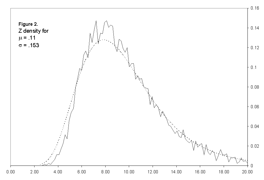
Figure 2: Comparison of Monte Carlo to Lognormal Fit
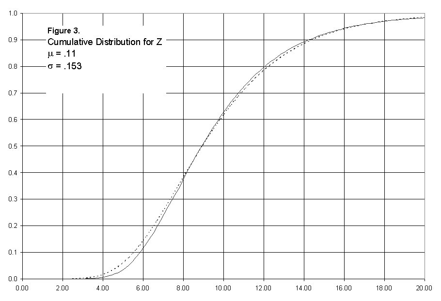
Figure 3: Cumulative Distribution for Z
So, for numerical purposes we are justified in assuming that Z is exactly
lognormal, of the form
![]()
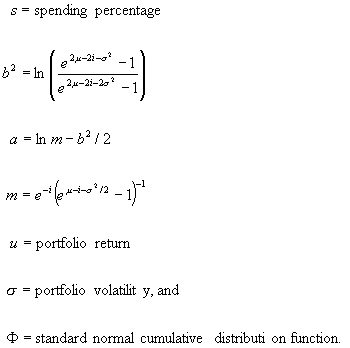
where e is a standard (0,1) normal random variable and some unknown constants a and b. Knowing the mean and variance of Z, we can solve for a and b. To do that we use the relationships

So we have,
![]()
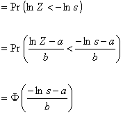
where

Plots of this for various values of s and our standard five portfolios are shown in Figure 1.
REFERENCES
Brunel, J. (1998): A Second Look at Absolute Returns, Journal Of Private Portfolio Management, Vol. 1, No. 1.
Benartzi, S. and Thaler, R. H. (1995): Myopic Loss Aversion and the Equity Premium Puzzle, Quarterly Journal of Economics, pp. 73-92.
McCabe, B. J. (1999): Monte Carlo Analysis of the Impact of Portfolio Volatility on After-Tax Wealth, to appear in Journal of Private Portfolio Management.
Johnson, N. L. and Kotz, S. (1970): Continuous Univariate Distributions
– 1, Houghton Mifflin.
Bernard McCabe is a Senior Vice President with the consulting firm Daniel H. Wagner Associates in Malvern PA. He was part of the team who developed R$P, a retirement planning program which considers uncertainty in portfolio returns.